


Next: Conclusion
Up: Two Theorems by Helmholtz
Previous: Applications
There is another important result by Helmholtz in the same paper we
mentioned
above. It concerns the most general infinitesimal deformation of a plastic
(that is, non-rigid) body.2
Consider a small volume element of a deformable body (a fluid, say).
Putting the origin of the coordinates inside this volume element,
let  be the position of a generic point
  . The
origin is denoted by
. The
origin is denoted by  . After a deformation,
the material point has a new position vector,
. After a deformation,
the material point has a new position vector,
 .
Also the point of the body located at the origin moved, its position
now being given by
.
Also the point of the body located at the origin moved, its position
now being given by  . We assume, as physically reasonable,
that
. We assume, as physically reasonable,
that  is, as a function of position, continuous and
differentiable to any order. In what follows, in order to get results
of enough generality, we assume very close to , that is to say,
we consider an infinitesimal volume of the body. Notice that
itself doesn't have to be small in what follows, though, in considering
deformations, this is somewhat academic, as finite deformations can always
be obtained from infinitesimal ones (for instance, by Lie group methods). This
notwithstanding, the geometrical interpretation we will get is only clear
for infinitesimal . On the other hand, the application for the
electric field which is done below would be impoverished by confining
to be infinitesimal.
A Taylor expansion for gives
is, as a function of position, continuous and
differentiable to any order. In what follows, in order to get results
of enough generality, we assume very close to , that is to say,
we consider an infinitesimal volume of the body. Notice that
itself doesn't have to be small in what follows, though, in considering
deformations, this is somewhat academic, as finite deformations can always
be obtained from infinitesimal ones (for instance, by Lie group methods). This
notwithstanding, the geometrical interpretation we will get is only clear
for infinitesimal . On the other hand, the application for the
electric field which is done below would be impoverished by confining
to be infinitesimal.
A Taylor expansion for gives
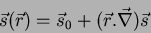 |
(14) |
neglecting further corrections, what is allowed by the restriction to
infinitesimal volume. Here we wrote for
 . In more detail, if
  is the
i-th component of , one has
is the
i-th component of , one has
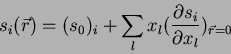 |
(15) |
This can be abbreviated to
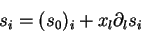 |
(16) |
or,
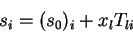 |
(17) |
where, obviously,
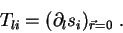 |
(18) |
In order to analyse this deformation in terms of more basic ones,
let us decompose  in the following way:
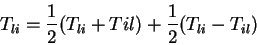 |
(19) |
and consider separately the symmetric and the antisymmetric parts.
The antisymmetric part is
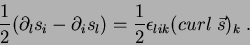 |
(20) |
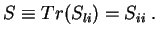
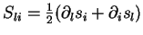
The symmetric part is
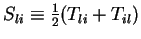 .
It can be decomposed as follows:
.
It can be decomposed as follows:
 |
(21) |
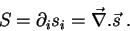
where
 Now,
Now,
 , so
that
, so
that
 |
(22) |
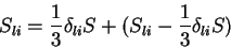
We can therefore write Eq.(21) as
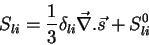 |
(23) |
where  is a traceless symmetric tensor.
Going now to Eq.(17), we can write
is a traceless symmetric tensor.
Going now to Eq.(17), we can write
 |
(24) |
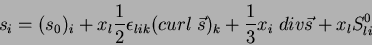
or,
 |
(25) |
where the last term is a vector whose i-th component is  . An
object
like
. An
object
like  is sometimes called a dyadic.It is a second-order tensor. Let
us examine
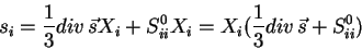
the meaning of the several terms of Eq.(25). The first term of
the
second member is a translation. The second is an infinitesimal rotation
around
the axis
is sometimes called a dyadic.It is a second-order tensor. Let
us examine
the meaning of the several terms of Eq.(25). The first term of
the
second member is a translation. The second is an infinitesimal rotation
around
the axis
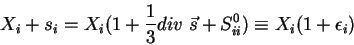
 , and the remaining terms describe
a dilatation
of the volume element. To understand them better, let us suppose
temporarily that
the translation and the rotation vanish, so that we have, for a component
of :
, and the remaining terms describe
a dilatation
of the volume element. To understand them better, let us suppose
temporarily that
the translation and the rotation vanish, so that we have, for a component
of :
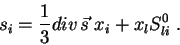 |
(26) |
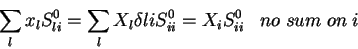
Now, is a symmetric matrix, so it can be diagonalized. This
means that
we can change coordinate axes in such a way that, in the new ones, the
matrix elements
of  have the form
 , where no sum is
implied
in this last expression. So, if the new coordinates are denoted by
, where no sum is
implied
in this last expression. So, if the new coordinates are denoted by  ,
we have
,
we have
 |
(27) |
so that
 |
(28) |
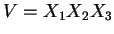
Consider the infinitesimal ``cube'' centered at , with as a vertex.
(The ``cube'' may have curvilinear edges, at least after the
deformation).
Its volume before the deformation was, in the new coordinates,
 . After the deformation, it is
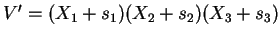 .
As we have, considering only the dilatation,
.
As we have, considering only the dilatation,
 |
(29) |
then
 |
(30) |
and, for the volume,
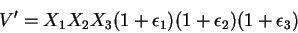 |
(31) |
which, to first order is
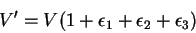 |
(32) |
that is,
 |
(33) |
but, as  is traceless,
 |
(34) |
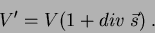
So, the do not contribute to the change of volume, but do
contribute to the change of the form of the little cube.
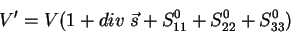
Referring again to Eq.(25), we see that is written
as a sum of a translation, plus a rotation, plus an isotropic dilatation,
plus a volume-conserving deformation.3
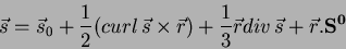
Notice that Eq.(25) was obtained using only Calculus. So, it should
apply to any vector field whatsoever. To shed more light on the role of each
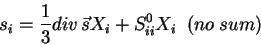
term of the expansion, let us use it for the electric field. We then have:
![\begin{displaymath}
\vec{E}(\vec{r})=\vec{E}(\vec{0}) + \frac{\vec{r}}{3}(div\,...
...{2}[(curl\,\vec{E})_0\times \vec{r}]
+ \vec{r}.{\bf S}^0
\;.
\end{displaymath}](img84.png) |
(35) |
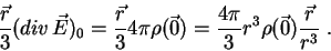
As
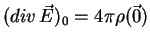 , the second term reads
 |
(36) |
Now, this is the field of a uniformly charged sphere of radius  at a point
of its surface. It is a radial field to be added to
at a point
of its surface. It is a radial field to be added to  .
The second term vanishes if the fields are static. Otherwise,
.
The second term vanishes if the fields are static. Otherwise,
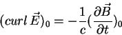 |
(37) |
and
![\begin{displaymath}
\frac{1}{2}[(curl\,\vec{E})_0\times \vec{r}]=-\frac{1}{2c}\frac{
\partial}{\partial t}[\vec{B}(\vec{0})\times\vec{r}]\;.
\end{displaymath}](img90.png) |
(38) |
Consider a uniform magnetic field of value
 . A
vector potential corresponding to it is
. A
vector potential corresponding to it is
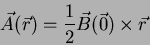 |
(39) |
so that we have
![\begin{displaymath}
\frac{1}{2}[(curl\,\vec{E})_0\times \vec{r}]=-\frac{1}{c}
\frac{\partial \vec{A}}{\partial t}\;.
\end{displaymath}](img93.png) |
(40) |
This means that the third term of (35) is the contribution
of the magnetic field at the origin, treated as follows: extend the value
of  at
at  to a uniform field. Compute its vector potential
and then add the term
to a uniform field. Compute its vector potential
and then add the term
 to
to
 . All the rest of the field at (and that could
be a lot!) comes from the term
. All the rest of the field at (and that could
be a lot!) comes from the term  .
.
Next: Conclusion
Up: Two Theorems by Helmholtz
Previous: Applications
Henrique Fleming
2002-04-15